6 Point on a circle
The coordinates \((x, y)\) of a point on a circle centered at the origin and having radius \(r\) are given by:
\[ \begin{eqnarray*} x & = & r \cos (\theta)\\ y & = & r \sin (\theta)\\ \end{eqnarray*} \]
where \(\theta\) is the angle measured from the positive \(x\)-axis.
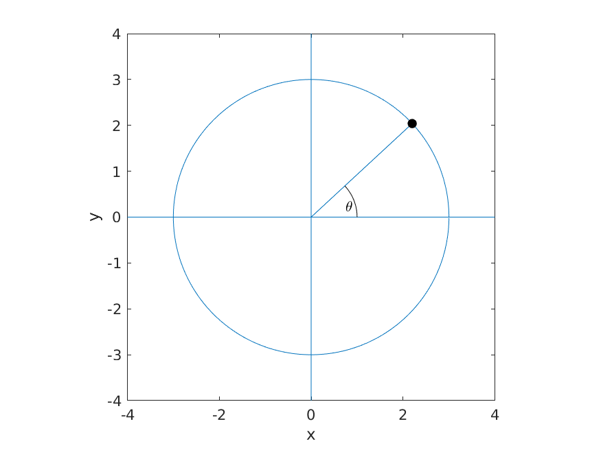
Figure 6.1: A circle of radius 3. The black point indicates a point on the circle at an angle of \(\theta\).
In MATLAB, open the file pointOnCircle.m. This file contains a user-defined function that when completed returns the coordinates of the point \((x, y)\) located at an angle of \(\theta\) on a circle having radius r.
Complete the function remembering to save the file every time that you edit it.
6.1 Using pointOnCircle.m
Test your function by typing the following in the MATLAB Command Window:
theta = pi / 3;
r = 1;
[x, y] = pointOnCircle(theta, r)
A correct function would cause the following to be output:
x =

    0.5000


y =

    0.8660
If the correct value is not output, review your function and correct any errors that you find.
Test your function using different values for the radius and \(\theta\); for example, type following statements in the MATLAB Command Window and verify that the outputs are correct:
[x, y] = pointOnCircle(0, 5.25)
[x, y] = pointOnCircle(pi / 2, 5.25)
[x, y] = pointOnCircle(pi, 5.25)
[x, y] = pointOnCircle(1.5 * pi, 5.25)
6.2 Plot a circle using pointOnCircle.m
We can generate multiple points on a circle with the following MATLAB code:
% 37 evenly spaced values between 0 and 2pi
theta = linspace(0, 2 * pi, 37);

% circle radius
radius = 3;

% pointOnCircle works with a vector of values for theta
[x, y] = pointOnCircle(theta, radius);
We can plot the points defined by the vectors x and y to produce the following figure:
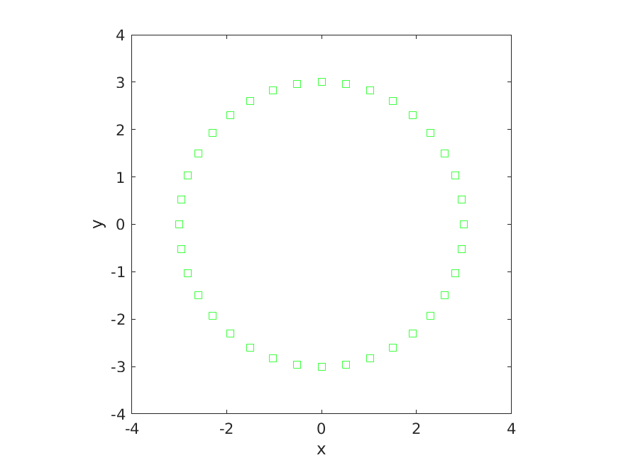
Figure 6.2: Three normal probability density functions having different mean values.
In MATLAB, open the file plotCircle.m. This file contains a script that when completed should generate the identical figure to that shown above.
To produce the circle shown above, we use the following steps:
- plot the points in
xandyusing green squares - set the aspect ratio of the axes so that equal tick mark increments on the x- and y-axis are equal in size
- set the limits of the x and y axes
- label the x-axis
- label the y-axis
Each one of the five steps shown above is accomplished using a different MATLAB function (Steps 2 and 3 are accomplished using the same function but using different input values for the function). The functions that you need to use in the order that you need to use them are:
plotaxisaxisxlabelylabel
Read the documentation for each function to determine how to use the function to accomplish each of the five steps required to generate the plot. You can use the help facility in MATLAB to easily determine how to accomplish each of the five steps:
help plothelp axishelp xlabelhelp ylabelComplete the script plotCircle.m and run the script to verify that it produces a plot identical to the one shown above.
More detailed information on each of the functions can be found uisng the links to the documentation below; note that there might be too much information for beginners to easily digest if you use the online documentation: