EECS4421/5324 Lab 04
Due: Friday March 16 before end of class
Introduction
In this lab we will experiment with the velocity and odometry motion models. We will try to replicate some of the figures shown in the lecture slides using an implementation of the velocity motion model. You will then implement the odometry motion model to replicate some of the figures for the odometry model shown in the lecture slides.
Velocity Motion Model
Copy and save the following Matlab functions.
vmotion.m: velocity motion model
function p = vmotion(xt, ut, xs, alpha, dt)
% VMOTION Velocity motion model
% Implements the velocity motion model described in Table 5.1
% of the textbook. All vectors are column vectors, and all angles
% are in radians.
%
% xt    - state at time t
% ut    - control at time t (linear and angular velocities)
% xs    - state at time t-1
% alpha - noise coefficients
% dt    - time step duration
%
% p     - probability density


% state variables at time t
xprime = xt(1);
yprime = xt(2);
thetaprime = xt(3);

% state variables at time t-1
x = xs(1);
y = xs(2);
theta = xs(3);

% control at time t
v = ut(1);
omega = ut(2);

mu = 0.5 * ((x - xprime)*cos(theta) + (y - yprime)*sin(theta)) / ...
           ((y - yprime)*cos(theta) - (x - xprime)*sin(theta));

xstar = 0.5 * (x + xprime) + mu * (y - yprime);

ystar = 0.5 * (y + yprime) + mu * (xprime - x);

rstar = sqrt((x - xstar)^2 + (y - ystar)^2);

dtheta = atan2(yprime - ystar, xprime - xstar) - ...
         atan2(y - ystar, x - xstar);

vhat = (dtheta / dt) * rstar;

omegahat = (dtheta / dt);

gammahat = (thetaprime - theta) / dt - omegahat;

% noise variances
sv = alpha(1) * v^2 + alpha(2) * omega^2;
somega = alpha(3) * v^2 + alpha(4) * omega^2;
sgamma = alpha(5) * v^2 + alpha(6) * omega^2;

p = mvnpdf(v - vhat, 0, sv) * mvnpdf(omega - omegahat, 0, somega) * ...
    mvnpdf(gammahat, 0, sgamma);
samplevmotion.m: sample from the velocity motion model
function xt = samplevmotion(ut, xs, alpha, dt, n)
% SAMPLEVMOTION Sample from the velocity motion model
% Implements the motion model sampling algorithm described in
% Table 5.3 of the textbook. All vectors are column vectors and
% all angles are in radians.
%
% ut    - control at time t (linear and angular velocities)
% xs    - state at time t-1
% alpha - noise coefficients
% dt    - time step duration
% n     - the number of samples to generate
%
% xt    - a 3xn matrix of sampled states (each column representing
%         a separate sample)

xt = zeros(3, n);
for a = 1:n
  % state variables at time t-1
  x = xs(1);
  y = xs(2);
  theta = xs(3);

  % control at time t
  v = ut(1);
  omega = ut(2);

  % noise variances
  sv = alpha(1) * v^2 + alpha(2) * omega^2;
  somega = alpha(3) * v^2 + alpha(4) * omega^2;
  sgamma = alpha(5) * v^2 + alpha(6) * omega^2;

  % generate noisy velocities
  vhat = v + mvnrnd(0, sv);
  omegahat = omega + mvnrnd(0, somega);
  gammahat = 0 + mvnrnd(0, sgamma);

  % ratio of linear to angular velocities
  f = vhat / omegahat;

  xprime = x - f*sin(theta) + f*sin(theta + omegahat*dt);
  yprime = y + f*cos(theta) - f*cos(theta + omegahat*dt);
  thetaprime = theta + omegahat*dt + gammahat*dt;

  xt(:,a) = [xprime; yprime; thetaprime];

end
pglobal.m: computes the motion model over a range of states in a fashion suitable for contour plotting
function [P, X, Y] = pglobal(xt, ut, xs, alpha, dt)
% PGLOBAL Evaluate the motion model over a range of states.
% [P, X, Y] = pglobal(xt, ut, xs, alpha, dt) computes the approximate
% position probability density over a range of states; it does so in
% such a way that generating a contour plot of the density is simple.
%
% You should first generate many samples using SAMPLEVMOTION and then
% pass the results to PGLOBAL.
%
% X and Y are matrices of x and y coordinates suitable for use in the
% CONTOUR family of functions.

xmin = min(xt(1,:));
xmax = max(xt(1,:));
dx = (xmax - xmin) / 40;

ymin = min(xt(2,:));
ymax = max(xt(2,:));
dy = (ymax - ymin) / 40;

zmin = min(xt(3,:));
zmax = max(xt(3,:));
dz = (zmax - zmin) / 100;


[X,Y,Z] = meshgrid(xmin:dx:xmax, ymin:dy:ymax, zmin:dz:zmax);
[nx, ny, nz] = size(X);
P = zeros(size(X));
for ix = 1:nx
   for iy = 1:ny
      for iz = 1:nz
         x = X(ix, iy, iz);
         y = Y(ix, iy, iz);
         theta = Z(ix, iy, iz);
         P(ix, iy, iz) = vmotion([x y theta]', ut, xs, alpha, dt);
      end
   end
end
X = X(:,:,1);
Y = Y(:,:,1);
P = sum(P, 3);
Produce Some Figures Using the Velocity Motion Models
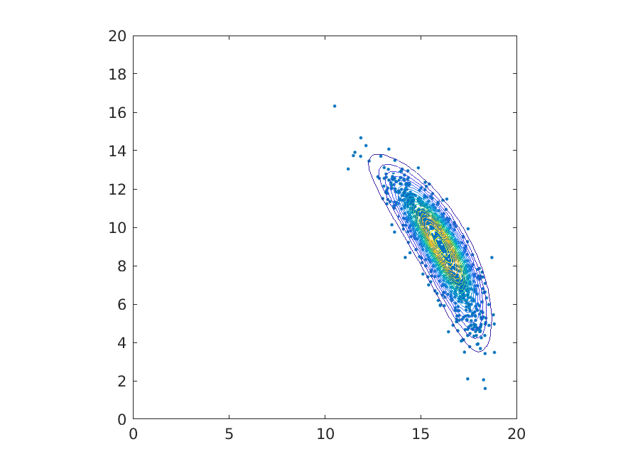
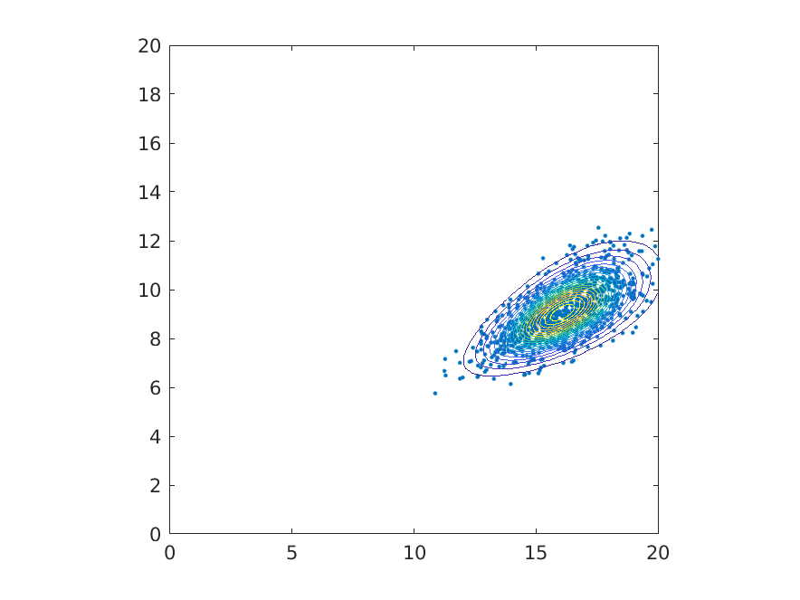
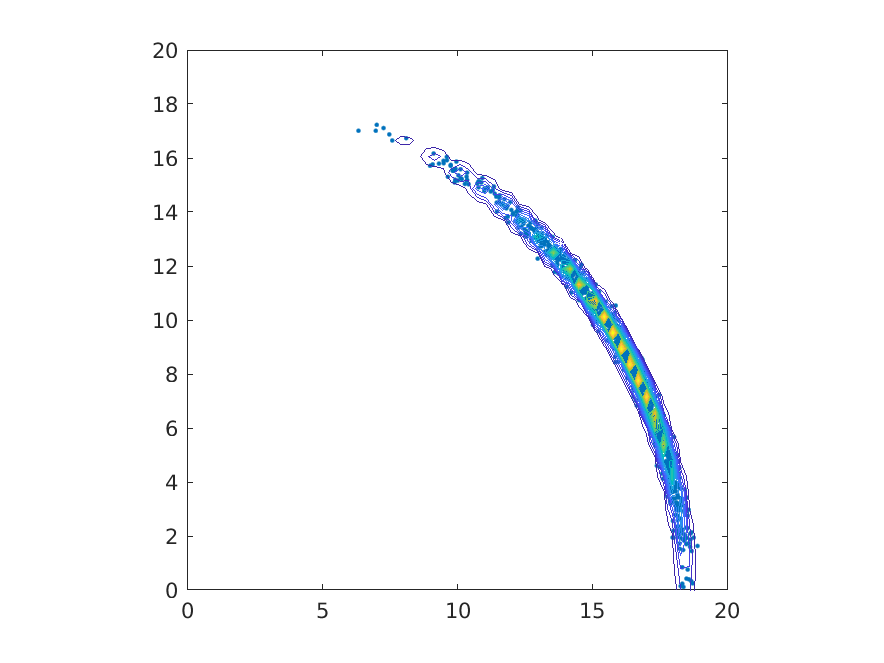
The following script shows you how to replicate the left-most figure from Slide 14 of "Odometry motion model.pdf" (the slides cover both the velocity and odometry models).
% start at origin facing to right
xs = [0; 0; 0];

% v = 1 m/s, w = 5 deg/s
ut = [1; 5*pi/180];

% noise coefficients
% left-most figure from Slide 14
alpha = [4 4 2 2 0.1 0.1] * 1e-4;

% middle figure from Slide 14
% alpha = [50 50 0.1 0.1 0.1 0.1] * 1e-4;

% right-most figure from Slide 14
% alpha = [1 1 8 8 0.1 0.1] * 1e-4;

% time step
dt = 20;

% sample the motion model and plot the results
xt = samplevmotion(ut, xs, alpha, dt, 1000);
plot(xt(1,:), xt(2,:), '.');
axis equal
hold on

% now evalate the density of the motion model over the range of xt
% and plot the results
[P, X, Y] = pglobal(xt, ut, xs, alpha, dt);
contour(X, Y, P, 20)
hold off
axis([0 20 0 20])
By adjusting the values of alpha you should be able to produce figures similar to the middle and right-most figures from Slide 14 (comment and uncomment the appropriate line to set alpha).
Implement the Odometry Motion Model and Sampling Algorithm
Implement the odometry motion model (Slide 35) and its accompanying sampling algorithm (Slide 26) and try to produce figures similar to those shown on Slide 36. Sample figures and parameter values are shown below:
xs = [0; 0; -20*pi/180];
ut = [0; 0; 0; 12; 14; 80*pi/180];
alpha = [0.5 0.5 10 1] * 1e-4;
xs = [0; 0; -20*pi/180];
ut = [0; 0; 0; 12; 14; 80*pi/180];
alpha = [0.05 0.05 100 10] * 1e-4;
xs = [0; 0; -20*pi/180];
ut = [0; 0; 0; 12; 14; 80*pi/180];
alpha = [2 2 1 10] * 1e-4;
Submission instructions
Submit the Matlab files needed to run your solution for the odometry motion model and the odometry sampling algorithm.
submit 4421 lab4 <your files>
You can also submit using websubmit
Graduate students, please hand in your solution to the written problem.