CSE1541 Lab 08
Line and polynomial fitting
Tue Mar 18, 2014
Due: Mon Mar 31 before 11:59PM
Introduction
This lab has you solve some simple polynomial and line fitting problems. There is an extended deadline for this lab because of the test next week.
You should put all of the MATLAB code for this lab in a single script.
Question 1: Chapter 14, Exercise 14 from the textbook
You can use this data file snowd.dat for the
question; the file contains the depth of snow in millimeters for 15 weeks
of measurements. To find the roots of the quadratic, you can use the MATLAB function
roots.
Question 2: The Vostok ice core samples
Vostok Station is a Russian research station in Antarctica which has recently been in the news for drilling into Lake Vostok, a subglacial lake located approximately 4,000 meters below the surface and thought to have been sealed off for about 15,000,000 years. The station is also famous for providing ice core samples that have been analyzed to estimate climate data dating back 420,000 years.
Download and save this data file which is modified version of the file http://physics.info/curve-fitting/vostok.txt. The data file has been created from information from the National Oceanic and Atmospheric Administration National Climatic Data Center.
From http://physics.info/linear-regression/problems.shtml: "Snow rarely gets a chance to melt in Antarctica, even in the summer when the sun never sets. In the interior of the continent, the temperature of the air hasn't been above the freezing point of water in any significant way for the last 900,000 years. The snow that falls there accumulates and accumulates and accumulates until it compresses into rock solid ice — up to 4.5 km thick in some regions. Since the snow that falls is originally fluffy with air, the ice that eventually forms still holds remnants of this air — very, very old air. By examining the isotopic composition of the gases in carefully extracted cores of this ice we can learn things about the past climatic conditions on earth. By extension we might also predict some things about the climate of the future. The columns in this data set are as follows:"
- age of the air sample (in years before the present time period)
- estimated temperature difference from the average temperature at Vostok during the current time period
- carbon dioxide concentration in parts per million
- dust concentration in parts per million
For this question, create a script that performs the following analysis on the Vostok data:
- Read in the data using
textread; you should replace missing values withNaN - Plot the estimated temperature difference versus age, and the CO2 level
versus age on the same graph using the function
plotyy; you will find the web-based documentation http://www.mathworks.com/help/matlab/ref/plotyy.html to be very useful, especially the first two examples. You should be able to reproduce Figure 1 shown below. Notice that the trend in temperature difference and CO2 levels seem to follow each other quite closely. - In a new figure, create a scatter plot the temperature difference versus
CO2 level using the MATLAB function
scatter. You should be able to reproduce Figure 2 shown below. - Notice that the relationship between CO2 level and temperature difference
is approximately linear (although very noisy). Use
polyfitto fit a straight line to the measurements, and then usepolyvalto evaluate the best fit line at 20 evenly spaced points from 150 to 350 parts per million of CO2. Plot the best fit line on top of the scatter plot to reproduce Figure 3 shown below. - Use
polyvalto extrapolate the temperature difference using the current level of atmospheric CO2 which is approximately 400 parts per million. - The extrapolated temperature will be much
higher than actual temperature difference at Vostok over the past
few years. However, notice that many data points lie below the
best fit line. Compute the residual errors between the measured
temperature differences and the best fit line (use
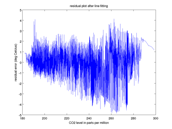
polyval). What is the smallest (most negative) residual error? What is the largest (most positive) residual error? - A resisdual plot is a graph where the residual errors are plotted versus
the independent variable (in this case, CO2 level). Create a residual plot
for your best fit line; you should be able to reproduce Figure 4 below.
Note that you need to sort the CO2 levels and then plot the
residuals corresponding to the sorted CO2 values (see the MATLAB
function
sort). Minitab (the maker of statistical software) has a nice blog post on residual plots here. Notice that at the highest levels of CO2, the residual errors are not very random. - Now that you have computed the residual errors, it is easy to compute the coefficient of determination, which is usually called R2 (R-squared). R2 is a measure of how well the data points fit the straight line model. A value of R2 close to 1 suggests that the best fit line closely fits the measured data; a value close to 0 suggests that there is no linear relationship between the dependent and independent variables (the temperature difference and CO2 levels, respectively). Compute R2 for the Vostok data by following the example here: http://www.mathworks.com/help/matlab/data_analysis/linear-regression.html
Figure 1:
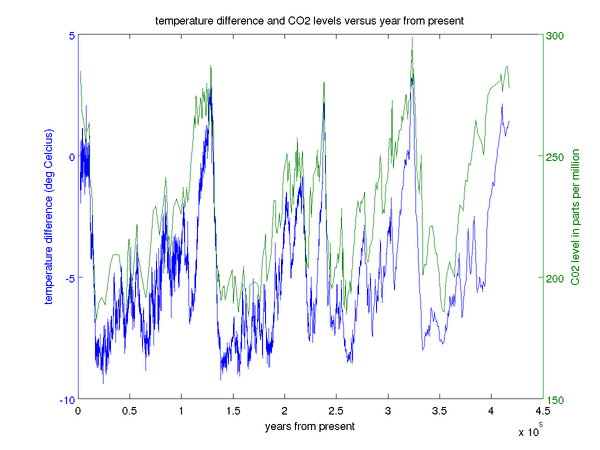
Figure 2:
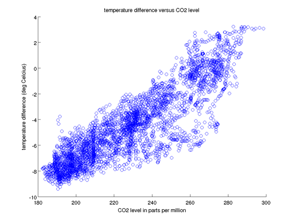
Figure 3:
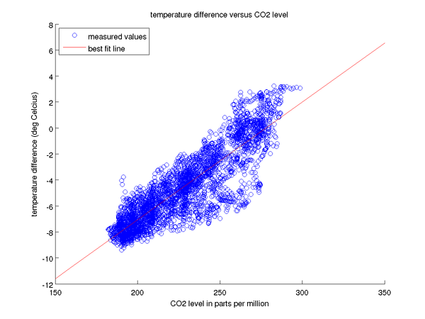
Figure 4:
Submit
You should have 1 script to submit.
Submit your file using the online submit service: https://webapp.eecs.yorku.ca/submit/