CSE1541 Lab 05

Introduction

This lab has you implement several different functions requiring if statements and loops. The first two questions are from the textbook; start from Question 3 if you did not bring a copy of the textbook.

Each question requires you to show some result using the function created in the question; you should put the MATLAB code that shows the results in a single script.

Question 1

Chapter 4, Exercise 35. Show that your function is correct by running the example in the question.

Question 2

Chapter 5, Exercise 29. To answer this question, first create a function named maximum that finds the largest element in a vector; start with the function definition shown below. Your function should use a loop with an if statement to find the largest element (i.e., do not use any MATLAB functions to find the largest element). Once you have created your function, use your function to answer the question.

function y = maximum(x)
%MAXIMUM Largest element in a vector
%  Y = MAXIMUM(X) returns the largest element in X.


end

Question 3

The Collatz conjecture is a famous unsolved mathematical problem. Start with some positive integer number and repeatedly apply the following rule until you reach the number 1:

If the number is even, divide it by 2.
If the number is odd, triple it and add 1.

The Collatz conjecture states that you will always reach the number 1 for any starting value; however, no one has yet proven or disproven the conjecture.

Write a function that computes the sequence of numbers using the rule for the Collatz conjecture. Start with the following function definition:

function seq = collatz(x)
%COLLATZ Collatz sequence
%  SEQ = COLLATZ(X) returns the sequence of numbers SEQ
%  for the Collatz conjecture starting from the positive
%  integer number X.


end

Use your function to plot the maximum value of the Collatz sequences starting from the numbers 1, 2, 3, ..., 100.

Question 4

A random walk is a path created by a succession of random steps. Physicists have used random walks to model physical phenomenon such as the motion of molecule in a liquid or gas (i.e., diffusion and Brownian motion).

A simple kind of random walk in 1-dimension can be described as follows. Start with a current value of zero. Flip a coin N times. Each time you flip the coin:

Add 1 to the current value if the coin shows heads.
Subtract 1 from the current value if the coin shows tails.

Write a function that computes the sequence for the random walk described above. Use the MATLAB function rand to simulate flipping a coin. Start with the following function definition:

function [y, seq] = walk1(n)
%WALK1 Random walk in 1-dimension
%  Y = WALK1(N) returns the last value in a 1-dimensional
%  random walk after N steps.
%
%  [Y, SEQ] = WALK1(N) also returns the sequence of N values
%  along the random walk.
%
%  The number of steps is optional. WALK1() uses N=100 steps.

end

Use your function to generate 1000 random walks of length 100. Plot a histogram of the last step for the 1000 walks. What kind of distribution does the histogram look like?

Question 5

Conway's Game of Life is a famous mathematical simulation that created an entire field of mathematics and computer science called cellular automata. The simulation is performed on a regular array where each element of the array (called a cell) has one of two possible states: alive or dead. A cell is aware of its 8 immediate neighbouring cells. The simulation proceeds one step at a time by following only four rules applied to all cells simultaneously:

A cell that is alive dies if it has fewer than two neighbours that are alive (as if caused by under-population)
A cell that is alive remains alive if it has two or three neighbours that are alive.
A cell that is alive dies if it has more than three neighbours that are alive (as if caused by over-population)
A cell that is dead becomes alive if it has exactly three neighbours that are alive (as if by reproduction)

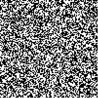
Although the simulation follows very simple rules, it is very difficult to predict the pattern of cells that will emerge. The image below shows 500 generations starting from a random pattern of cells.

Write a function that computes one generation of Conway's Game of Life. Start with the function definition shown at the end of this question which contains a local function named alive that computes the number of cells that are alive in the neighbourhood of the cell A(row, col). To test your function, create some of the patterns shown in the Wikipedia page http://en.wikipedia.org/wiki/Conway%27s_Game_of_Life#Examples_of_patterns:

Create a "Beehive" pattern in a 5x6 array and show 1 generation (i.e., call your function once); the pattern should remain unchanged. If your pattern is stored in an array named A then you can show the pattern using the function imshow:
```
% shows A as an image magnified by 1000 percent
imshow(A, 'InitialMagnification', 1000);
```
Create a "Blinker" pattern in a 5x5 array and show 5 generations; the pattern should oscillate between a vertical and horizontal bar.
Create a "Glider" pattern in a 20x20 array and show 50 generations; the pattern should move down and left in the array. It will be useful to generate a movie of the Glider because there are many generations. If your pattern is stored in an array named A then you can make and play a movie of your glider like so:
```
clear F;
F(50) = struct('cdata',[],'colormap',[]);
for j = 1:50
  imshow(A, 'InitialMagnification', 1000);
  A = conway(A);
  F(j) = getframe;
end
movie(F)
```

Start with the code below:

function B = conway(A)
%CONWAY One generation of Conway's Game of Life.
%  B = CONWAY(A) computes the next generation B starting from
%  the current generation A using the rules of Conway's
%  Game of Life.
%
%  A is a 2-dimensional array of values where the value
%  0 indicates that the cell is dead, and any other value indicates
%  that the cell is alive.



end


function n = alive(A, row, col)
%ALIVE Number of neighbours that are alive.
%  N = ALIVE(A, ROW, COL) returns the number of neighbours
%  that are alive surrounding the cell A(ROW, COL)

[nRows, nCols] = size(A);
startRow = max([row - 1, 1]);
stopRow = min([row + 1, nRows]);
startCol = max([col - 1, 1]);
stopCol = min([col + 1, nCols]);
neighbourhood = A(startRow:stopRow, startCol:stopCol);
n = sum(neighbourhood(:) > 0);
if A(row, col) > 0
  n = n - 1;
end

Submit

You should have 5 functions and 1 script to submit.

Submit your 6 files using the online submit service: https://webapp.eecs.yorku.ca/submit/

CSE1541 Lab 05 Selection statements and loops