CSE1541 Lab 04
Functions
Tue Jan 28, 2014
Due: Fri Feb 14 before 11:59PM
Introduction
This lab has you implement several different functions to solve various problems in physics.
Question 1
Create a function named dprod that has two parameters that
are both n-dimensional vectors, and returns the dot
product of two vectors. Your function should compute the
dot product using the mathematical definition (i.e., do not use the
built-in MATLAB function dot).
Check that your implementation is correct by comparing the results
of your function to the MATLAB function dot.
Question 2
Create a function named cprod that has two parameters that
are both 3-dimensional vectors, and returns the cross
product of two vectors. Your function should compute the
cross product using the mathematical definition (i.e., do not use the
built-in MATLAB function cross).
Check that your implementation is correct by comparing the results
of your function to the MATLAB function cross.
Question 3
This question is related to the phenomenon of exponential growth.
An Indian legend has it that the game of chess was invented by mathematician who showed his invention to his king. The king was so pleased with the game that he asked the mathematician to name the price for the invention. The mathematician said: "Take my chess board and place one grain of rice on the first square, then place two grains on the second square, then place four grains on the third square, and so on, doubling the number of grains for each new square, until all 64 squares have been processed. The total amount of rice will be my payment." The king accepted the offer.
Create a function named chessboard that has a single positive
integer parameter n. Your function should return two values:
the number of grains of rice on square number n, and the total
number of grains of rice on squares 1–n.
There is a simple formula for computing the total number grains; for this
exercise you should NOT use this formula. Instead, compute the number
of grains on squares 1–n and compute
the total using the MATLAB function sum.
You can read more about this problem by following this link.
Question 4
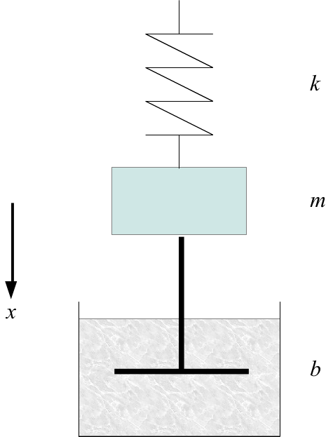
The diagram above illustrates an ideal damped harmonic oscillator
(a spring with spring constant k, a mass with mass
m, and a damping fluid with damping constant b).
The position x(t) of the mass as a function of time is given by:

where A is the amplitude of the motion and φ is the phase.
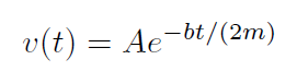
The envelope v(t) of the oscillation is simply the amplitude
times the exponential term:
Create a function named dhmotion that implements the
equations shown above. Your function should have 5 scalar parameters
(amplitude, mass, spring constant, damping
constant, phase) and 1 vector parameter of times. Your function should return
two vectors: the vector of positions x(t) evaluated at
each time in the input vector, and the vector of the exponential
envelope v(t) evaluated at
each time in the input vector.
Question 5
Create a script that uses the functions you created above to solve the following questions. You should be able to generate a nice looking report using your script.
5a Matrix multiplication
Use your function dprod to show how to compute the
matrix product A * B where A and B
are given by:
  A = [1 3; 4 2];
  B = [-1 5; -3 8];
5b Angular momentum
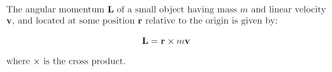
Use your function cprod to compute the angular momentum of
an object having the following:
  m = 1.5;
  r = [6 6 8];
  v = [-1 1 0];
5c Tabulate the amount of rice
Use your function chessboard, the function sprintf,
and the function disp to produce the following table of values:
square 1	grains 1	total 1
square 2	grains 2	total 3
square 3	grains 4	total 7
square 4	grains 8	total 15
square 5	grains 16	total 31
square 6	grains 32	total 63
square 7	grains 64	total 127
square 8	grains 128	total 255
square 32	grains 2.147484e+09	total 4.294967e+09
square 64	grains 9.223372e+18	total 1.844674e+19
In the table, the columns are separated using tabs.
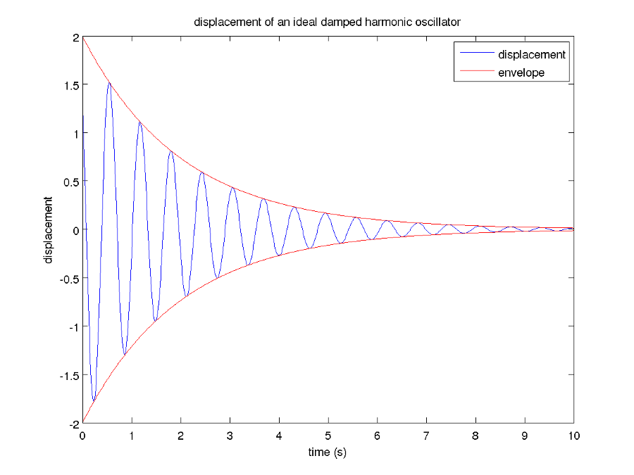
5d Plot the motion of a damped harmonic oscillator
Use your function dhmotion to plot the position
and both sides of the envelope for the following values:
A = 2;
m = 0.5;
k = 50;
b = 0.5;
phi = pi / 4;
t = linspace(0, 10, 1000);
You should get something similar to:
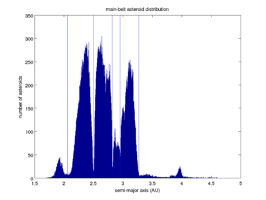
5e Kirkwood gaps
This question does not require the use of the functions you created.
Instead it requires you to use MATLAB's load function.
Save a copy of the file kirkwood.csv. The file contains
602,003 lines with one floating point number on each line. Each
number represents the length of the semi-major axis in astronomical units
(AU) of the orbit of a known asteroid in the asteroid belt.
Use the MATLAB function load to load the contents of the file
kirkwood.csv. Use the MATLAB function hist
to generate a histogram of the data (try using a variety of bin
sizes such as 10, 100, 1000, and 10000 to see the effect of bin size).
For a large enough number
of bins, you should see gaps in the histogram. These gaps are called
Kirkwood gaps, and are caused by interactions with the orbit of Jupiter.
You can find out more about the Kirkwood gaps using the following links:
Draw vertical lines on your histogram at the following values on the semi-major axis axis:
- 2.06 AU
- 2.5 AU
- 2.82 AU
- 2.95 AU
- 3.27 AU
These values are the locations of 5 of the Kirkwood gaps. You should get something similar to:
Submit
You should have 4 functions and 1 script to submit.
Submit your 5 files using the online submit service: https://webapp.eecs.yorku.ca/submit/