CSE1541 Lab 03

Introduction

This lab explores vector and matrix manipulation in MATLAB. In the first part of the lab, we use matrices to represent data namely, the three different pieces of data that are needed to draw a simple 2D geometric object. We use array manipulations to move the geometric object, and we use matrix multiplication to change the shape of the object. We then generalize our approach to a 3D shape.

The second part of the lab has you explore the various properties of the transformations that were discussed in the first part of the lab.

The third part of the lab consists of a variety of questions that cover manipulations and uses of arrays that were not covered in the lectures.

Part 1: Introduction to computer graphics

This is an in-lab demonstration. The purpose of this not-so-short demonstration is to illustrate MATLAB's patch command for drawing 2D and 3D polygons (or faces). The demonstration also illustrates the geometric transformations called translation, scaling, and rotation.

%% Lab 3

%% Drawing a 2D object

% The vertices of a square centered at the origin
% each row represents the coordinates of one vertex
V = [-1 -1;
      1 -1;
      1  1;
     -1  1];
 
% The face vector is a row vector that describes which vertices
% of V are used to form the perimeter of the face that we want to draw.
% In this case, we want to draw the square using the first,
% second, third, and fourth vertices of V:
F = [1 2 3 4];

% The color vector is the red-green-blue color for the face.
% We will draw a red square.
C = [1 0 0];

% Use the patch command to draw the square:
patch('Faces', F, 'Vertices', V, 'FaceVertexCData', C, 'FaceColor', 'flat');
axis([-8 8 -8 8])
axis square

%% Moving a 2D object

% To move an object, we add a translation vector to each vertex of
% the object. For example, we can move the square 4 units to the
% right by adding 4 to the x-component of each vertex:
W = V + [4 0; 4 0; 4 0; 4 0];
C = [0 0 1];
patch('Faces', F, 'Vertices', W, 'FaceVertexCData', C, 'FaceColor', 'flat');

% We can move the square 4 units up by adding 4 to the y-component of
% each vertex:
W = V + [0 4; 0 4; 0 4; 0 4];
C = [0 1 0];
patch('Faces', F, 'Vertices', W, 'FaceVertexCData', C, 'FaceColor', 'flat');

% We can move the square 4 units down and to the left by adding
% the vector [-4 -4]/sqrt(2) to each vertex in V:
d = [-4 -4] / sqrt(2);
D = repmat(d, [4 1]);
W = V + D;
C = [1 1 0];
patch('Faces', F, 'Vertices', W, 'FaceVertexCData', C, 'FaceColor', 'flat');

%% Rotating a 2D object

% To rotate an object around the origin by an angle of theta radians,
% we can multiply the vertices as column vectors by a rotation
% matrix R:
figure
C = [1 0 0];
patch('Faces', F, 'Vertices', V, 'FaceVertexCData', C, 'FaceColor', 'flat');
axis([-2 2 -2 2])
axis square

theta = 30*pi/180;
R = [cos(theta) -sin(theta);
     sin(theta)  cos(theta)];
W = R * V';
W = W';
C = [0 1 1];
patch('Faces', F, 'Vertices', W, 'FaceVertexCData', C, 'FaceColor', 'flat');

%% Scaling a 2D object

% To scale an object about the origin we can multiply the vertices
% as column vectors by a scale matrix S:
figure
C = [1 0 0];
patch('Faces', F, 'Vertices', V, 'FaceVertexCData', C, 'FaceColor', 'flat');
axis([-5 5 -5 5])
axis square

sx = 2;
sy = 2;
S = [sx 0;
     0  sy];
W = S * V';
W = W';
C = [1 0 1];
patch('Faces', F, 'Vertices', W, 'FaceVertexCData', C, 'FaceColor', 'flat');

% The scale factors do not need to be the same:
figure
C = [1 0 0];
patch('Faces', F, 'Vertices', V, 'FaceVertexCData', C, 'FaceColor', 'flat');
axis([-5 5 -5 5])
axis square

sx = 0.5;
sy = 2;
S = [sx 0;
     0  sy];
W = S * V';
W = W';
C = [1 0 1];
patch('Faces', F, 'Vertices', W, 'FaceVertexCData', C, 'FaceColor', 'flat');

%% Drawing a 3D object

% The vertices of a cube centered at the origin
% each row represents the coordinates of one vertex
V = [-1 -1  1;
      1 -1  1;
      1  1  1;
     -1  1  1;
     -1 -1 -1;
      1 -1 -1;
      1  1 -1;
     -1  1 -1];
 
 % The six faces of the cube. Each row are the of F are the row-indices
 % of V that define each face.
 F = [1 2 3 4;
      2 6 7 3;
      6 5 8 7;
      5 1 4 8;
      4 3 7 8;
      5 6 2 1];
  
 % The colors of the faces. Each row is the color of the corresponding
 % face in F.
 C = [1 0 0;
      0 1 0;
      0 0 1;
      1 1 0;
      1 0 1;
      0 1 1];

figure
patch('Faces', F, 'Vertices', V, 'FaceVertexCData', C, 'FaceColor', 'flat');
axis([-3 3 -3 3 -3 3])
axis square

Part 2: Investigate some properties of geometric transformations

Create a new script to answer Questions 1-8.

For Questions 1-8, the goal is to generate a report that clearly communicates a solution for each question. Your report should be publishable as a web page.

In your scripts, please show how you calculated your answers using MATLAB.

Question 1: Show that translations in 2D commute

Suppose that you translate the original square from the demo by a translation vector d₁ and then translate it again by a second translation vector d₂. Show that you get the same result if you first translate by d₂ and then translate by d₁. The clearest way to show this is to generate two separate figures (the first where you translate by d₁ followed by d₂, and the second where you translate by d₂ followed by d₁). Consider adding titles to your figures to communicate the order of the translations.

Question 2: Show that rotations in 2D commute

Suppose that you rotate the original square from the demo by an angle θ₁ and then rotate it again by a second angle θ₂. Show that you get the same result if you first rotate by θ₂ and then rotate by θ₁. As with Question 1, the clearest way to show this is to generate two separate figures with titles.

Question 3: Show that 2D transformations in general do not commute

Suppose that you translate the original square in the demo by a translation vector d₁ and then rotate it by an angle θ₁. Show that you get a different result if you first rotate by θ₁ and then translate by d₁. As with Question 1, the clearest way to show this is to generate two separate figures with titles.

Question 4: Show that 2D translation can be written as matrix multiplication

Show that the matrix equation for translation yields the same results as vector addition. Do this by first translating the original square from the demo by some translation vector d (just like we did in the first part of the lab). Next, in a separate figure, translate the original square using the matrix equation and show that you get the same result. Note that when using the matrix equation, you must append a 1 as the third component to each of the original vertices, and then you must use only the first two components of the transformed vertices.

Question 5: Show that a sequence of transformations can be written as matrix multiplication

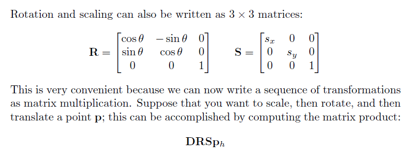
Show that the matrix equation for a sequence of transformations yields the same results as performing the transformations one at a time. Do this by first scaling the original square from the demo; then rotate the scaled square; finally, translate the scaled square. In a separate figure, use the matrix equation to transform the original square. Note that when using the matrix equation, you must append a 1 as the third component to each of the original vertices, and then you must use only the first two components of the transformed vertices.

*3D computer graphics uses the 3D version of the matrix formulation shown above to transform objects. Your video card has been designed to perform 4 × 4 matrix multiplication very fast.

Question 6: Show that rotations in 3D do not commute

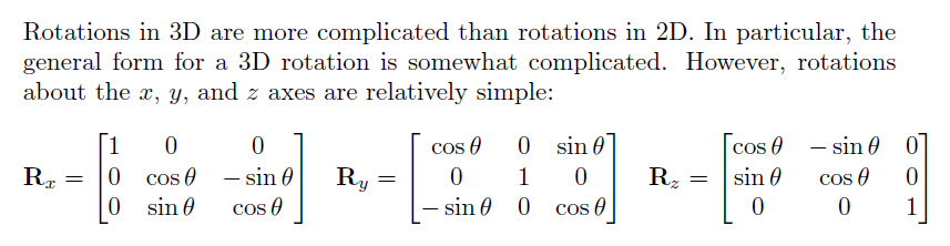
Suppose that you rotate the original cube from the demo about the z-axis by an angle θ₁ and then rotate it again about the y-axis by a second angle θ₂. Show that you get a different result if you first rotate the original cube about the y-axis by θ₂ and then rotate about the z-axis by θ₁. Note that the results are very obvious if you choose θ₁ = θ₂ = 90 degrees, and draw the faces of the cube using different colors like we did in the demo. Again, use two figures to show the two different results.

Part 3: Explore more manipulations and uses of matrices

Question 7: `fliplr` and `flipud`

Create the matrix:

A =
     1     2     3     4
     5     6     7     8

Using only the commands fliplr and flipud to manipulate the matrix A show how to obtain the following matrix:

ans =
     8     7     6     5
     4     3     2     1

Question 8: `reshape`

Create the matrix:

A =
     1     2     3     4
     5     6     7     8
     9    10    11    12

Using only the command reshape to manipulate the matrix A show how to obtain the following matrix:

Using only the transpose operator and the command reshape to manipulate the matrix A show how to obtain the following matrix:

ans =
     1     3     5     7     9    11
     2     4     6     8    10    12

Question 9

Do Exercise 40 from Chapter 3 of the textbook. For this question, you need to create a new script that you should call q9.m

You will need to read the textbook to find out how to prompt the user for input (or type help input or doc input in MATLAB).

Question 10

Do Exercise 41 from Chapter 3 of the textbook. For this question, you need to create a new script that you should call q10.m

You will need to read the textbook to find out how to prompt the user for input (or type help input or doc input in MATLAB).

Submit

You should have 3 scripts to submit: the script for Questions 1-8, q9.m, and q10.m

Submit your 3 scripts using the online submit service: https://webapp.eecs.yorku.ca/submit/

CSE1541 Lab 03 Matrices