CSE4421 Lab 06

Introduction

In this lab we will implement the Kalman filter SLAM simulation from yesterday's lecture. Before attempting this lab you should review the Kalman filter algorithm from the textbook (Table 3.1) and yesterday's lecture slides for the SLAM problem where all landmarks are measurable by the robot at every time step.

Kalman Filter SLAM

Copy and save the following Matlab script.

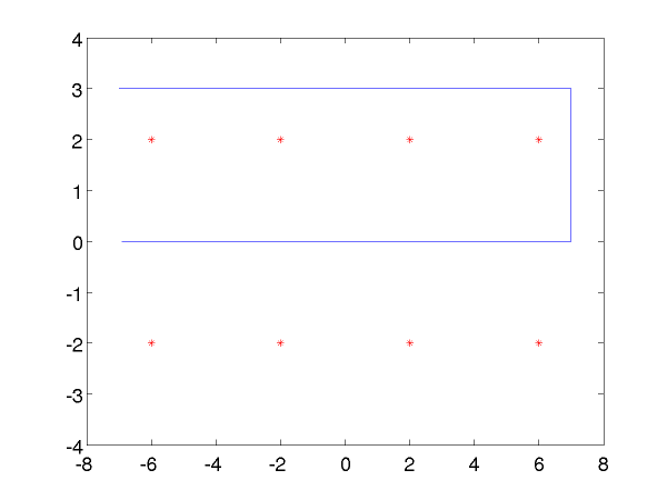
The script sets up the simulation of KF SLAM from yesterday's lecture. There are 8 point landmarks that the robot traverses in a rectangular path (see figure below). The true path and true (noise free) controls are stored in the variables X and U, respectively.

Your task is to complete the code in the for loop so that it generates a noisy control input and a noisy measurement of the landmark offsets for each iteration of the loop. Also, you need to implement the Kalman filter equations inside the loop where indicated. The amount of code that needs to be written is actually very small; the majority of the work lies in reading and understanding the code that has been supplied to you.

When you have finished implementing the code inside the loop, you should run the completed script. Plot the estimated path of the robot, the estimated covariance of the robot's position at several points along the path, and the estimated covariance of the landmarks after the robot has completed its tour around the landmarks. Because the noises are all isotropic in this simulation, the estimated covariances will also be isotropic. You can use the function named circle (shown below) to plot the covariance circles (ask if you do not know how to determine the radius of the circle to draw).

Time permitting, you might try implementing the other variations discussed in yesterday's lecture (measuring markers only within a certain distance to the robot, and loop closure).

% true landmark locations L as column vectors
L = [-6 -2  2  6 -6 -2 2 6;
     -2 -2 -2 -2  2  2 2 2];

% number of landmarks
nL = size(L, 2);

% true path waypoints as column vectors
w = [-7 7 7 -7 
      3 3 0  0];
      
% number of waypoints
nw = size(w, 2);

% true path X (connecting the waypoints) and true controls U
% stepsize is the distance the robot travels during each step
stepsize = 0.1;
X = [];
U = [];
for a = 1:(nw - 1)
    start = w(:, a);
    stop = w(:, a + 1);
    delta = stop - start;
    dist = norm(delta);
    delta = delta / dist;
    step = 1;
    X = [X start];
    U = [U [0 0]'];
    next = start + stepsize * delta;
    while norm(next - start) < dist
        X = [X next];
        U = [U [stepsize * delta]];
        step = step + 1;
        next = start + step * stepsize * delta;
    end
end
nX = size(X, 2);

% Kalman filter estimation of location and landmark locations

% state vector dimensions
xdim = 2 * nL + 2;

% storage for the estimated state x (at time t)
x = zeros(xdim, nX);
x(1:2, 1) = X(:,1);    % assume we know the starting location of the robot

% storage for the estimated state covariance Sigma (at time t)
Sigma = zeros(xdim, xdim, nX);
Sigma(:, :, 1) = 25 * eye(xdim);
Sigma(1:2, 1:2, 1) = 0.1 * 0.1 * eye(2);

% state transition covariance R
% this is all zeros except for the covariance of the control noise Ru
Ru = [0.05*0.05   0;
      0           0.05*0.05];
R = zeros(xdim, xdim);
R(1:2, 1:2) = Ru;

% measurement covariance Q
% assume each landmark measurement has noise covariance Qi
zdim = 2 * nL;
Qi= [0.2*0.2   0;
     0         0.2*0.2];
Q = 0.2 * 0.2 * eye(zdim);

% for each time step 2, 3, 4, ...
% time t = 1 corresponds to the initial state of the robot
for t = 2:nX
    % make a noisy control input ( use Ru as the noise covariance and
    % add zero-mean Gaussian noise to U(:, t-1) )

 
 
    % predict (lines 2 and 3 of Table 3.1)

 
 
    % make noisy measurements (use Qi for the noise covariance in an
    % individual landmark, or Q as the noise covariance for all of the
    % landmarks)

 
 
    % correct (lines 4, 5, and 6 of Table 3.1)
    % store mu_t in x(:, t)
    % store Sigma_t in Sigma(:, :, t)




end

circle.m: draw a circle

function h = circle(center, radius, col)
% CIRCLE Draw a circle
%
% H = CIRCLE(CENTER, RADIUS) draws a circle centered at
% CENTER with radius RADIUS using the color blue.
%
% H = CIRCLE(CENTER, RADIUS, COL) draws a circle using
% the color specified by COL.
%
% H is a handle to the circle object.

if nargin == 2
    col = 'b';
end    

delta = [-1 -1]';
pos = center(:) + radius * delta;
h = rectangle('position', [pos' 2*[radius radius]], ...
              'curvature', [1 1], ...
              'EdgeColor', col);

True path of robot